Can We Benefit from Temporal Features in Games for User Behaviour Prediction?
Background
For games, especially in free-to-play online games, it’s very important to predict users’ behaviors, such as their play-time, shopping cart preference, or churn probability and so on. Most online games need servers to sychronize users information, so it’s very easy to record, store and process user behavior data on server side, which needs sdk to record logs, data warehouse to store data and big-data suite to process information.
My major job is to predict user behaiors based on these data, metention above. In this blog, I will share a series of models to show the effectiveness of temporal features in games. The task is to predict whether user will churn 7 days after registering, which is a binary classification problem. The data is user actions, distributed in decades of tables, such as login table, purchase table, play-round table , etc. It uses AUC to evaluate the effectiveness of models.
Model 1: Bi-RSU
As to make use of temporal data, the first model is a simple Bi-directional GRU, short for Bi-GRU, model. Every time, a user logouts the game, it records the play-time of the user during this session. The Bi-GRU takes the logout play-time series and aggregates the temporal information. Then, a MLP layer is appended to discriminate the final objective, churn or not, as shown below.
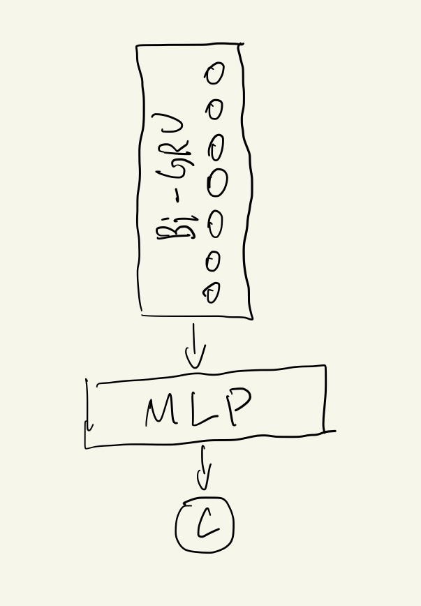
The AUC for Bi-GRU is 0.773. The total sample size is about 600,000, and churn rate is about 60%. The result is not bad, but It could get a better result. So, put mode 1 as a baseline.
Model 2: Model 1 plus more features
The system also stores user other information, besides play-time, when they logout at the same time, such as the hero level distribution in their package, the money they gained, the number of their in-game friends, etc. So, add the extra information in the same series to build the model 2, as following,
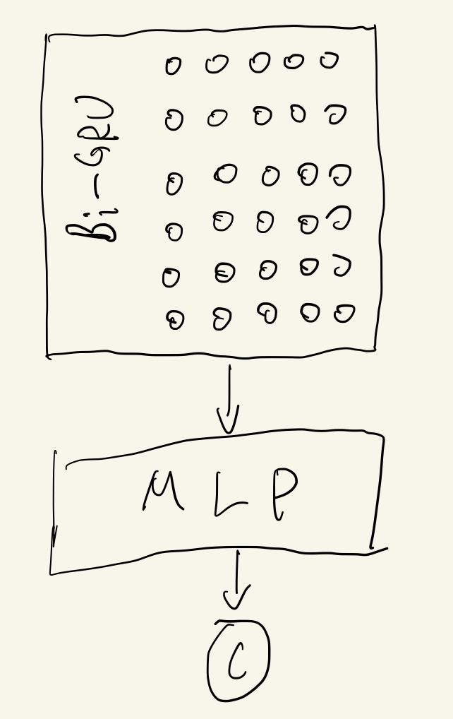
It is worthing noting that the all features are in the same temporal series. The model gets AUC 0.786, which there is a slight imporvement, compared to the previous model .
Model 3: Model 2 plus feature rescaling
As the model takes mulitple features, it should transform the features to avoid some specific features dominating the whole optimization process. For simplicity, use logrithm to rescale all features. I encourage you to try other normalization methods.
![]()
The AUC for this model is 0.817, which is very impressive. It also means that specific features dominating did occur in the last model.
Model 4: XGBoost with features engineering
In the previous model, we gained an impressive Bi-GRU model. Now, introduce a classic model, Xgboost. Our team has use xgboost for a while, as it’s very efficient and effectiveness. The algorithm has also dominiated many AI competitions around the world. However, there is an obvious drawback that xgboost cannot handle data with variable length, such as temporal series data. It needs great amounts of feature enginniering to transform them to stable length features. That’s why we are so interested in deep learning based methods, as they provides an end-to-end solution so that machine learning engineers would focus on the most important and interesting part of the problem .
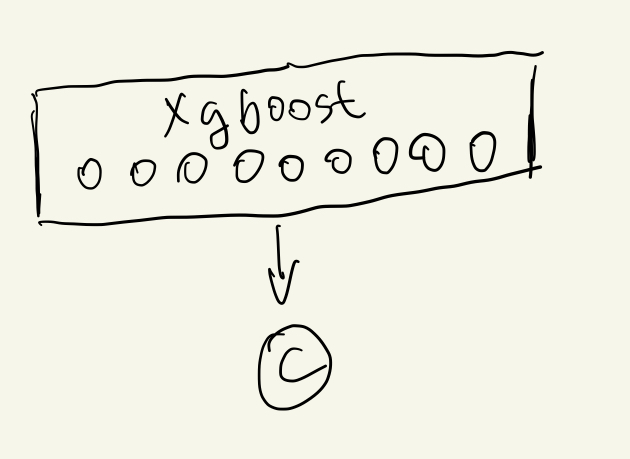
After some feature engineering, our xgboost model achieves AUC with 0.818, which is slight higher than model 3. It means that all we did before is useless. I don’t think so. The story of model evolution does not end. Let’s continue.
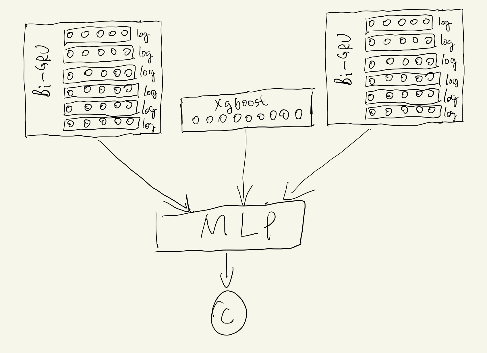
Model 5: Model 3 plus Model 4
Model 4 get a great result, which inspired us that we could make use of it and combines it with model 3. This is another reason that I like deep learning based method, because it is very flexible that it can change the structure as far as needed. The model 5 is as following, which merge sequence and aggregation information together.
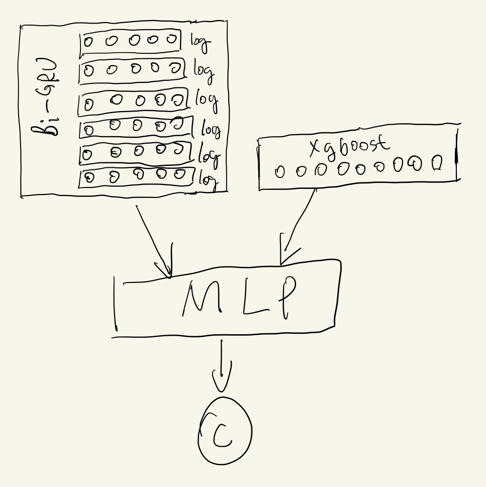
The AUC for model 5 is 0.843, which means that temporal features produced by Bi-GRU do work, and my assumption, as the title of the blog mentioned, is proven.
Model 6: Model 5 plus different embedding series
In model 6, it adds an extra temporal series, the improvment is slight, which is AUC 0.845.
That adding more series, and applying pretrained model , such Word2Vector or BERT, to embed each element in series might achieve better results, that is what we would do in the future.
Summary
We have run 6 models, and gained lift step by step. The improvement of AUC shows that temporal data can add extra information, campared with only aggregated features, to make the model more accurate. Of course, it need more experiemnts to demostrate the generalizability the effectiveness. This experiment give us some inspiration and we will follow up and apply it in the real world problem in the future. The table below collects all result recorded in this blog.
| Model | AUC |
|---|---|
| Model 1: Bi-RSU | 0.773 |
| Model 2: Model 1 plus more features | 0.786 |
| Model 3: Model 2 plus feature rescaling | 0.817 |
| Model 4: XGBoost with features engineering | 0.818 |
| Model 5: Model 3 plus Model 4 | 0.843 |
| Model 6: Model 5 plus different embedding series | 0.845 |
 支付宝打赏
支付宝打赏
 微信打赏
微信打赏
您的打赏是对我最大的鼓励!